2.2 李群流体流形（Lie-Manifolds）上的加权高斯-牛顿（最小二乘）优化方法 Weighted Gauss-Newton Optimization on Lie-Manifolds

Two images are aligned by Gauss-Newton minimization of the photometric error

which gives the maximum-likelihood estimator for $\mathbf{\xi}$ assuming i.i.d. Gaussian residuals.

两幅图像之间的配准，见公式（5）（就是最小二乘的优化问题，译者额外添加备注）可以认为是（以相机位姿 $\mathbf{\xi}$ 为自变量，单个光度测量误差项二次型是： $r_{i}^2(\mathbf{\xi})$ ，整体光度测量误差项二次型（photometric error）之和 $E(\mathbf{\xi})$ 为误差函数的，译者额外添加备注）用高斯—牛顿（迭代法）的优化问题，其目的就是要最小化（整个）光度测量误差项二次型（之和），假设图像上的（单个）光度测量误差项，是独立同分布（i.i.d.）的高斯分布残差（ Gaussian residuals），那么这个优化问题得到的结果，就是 $\mathbf{\xi}$ 的极大似然值（即：优化后的相机姿态，译者额外添加备注）。

We use a left-compositional formulation: Starting with an initial estimate $\mathbf{\xi}^{(0)}$ , in each iteration a left-multiplied increment $\delta\mathbf{\xi}^{(n)}$ is computed by solving for the minimum of a Gauss-Newton second-order approximation of $E$ :

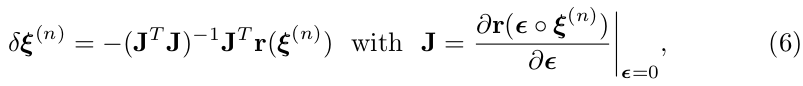
见公式（7），(高斯-牛顿迭代过程中) 使用一个左乘复合迭代函数（left-compositional formulation）：从初始估计（相机姿态变换） $\mathbf{\xi}^{(0)}$ 开始，（高斯-牛顿）每次迭代过程中，左乘更新量 $\delta\mathbf{\xi}^{(n)}$ ，这个更新量是通过（误差函数） $E$ 的高斯-牛顿二阶近似求解的最小值得到的：（如下公式6）

where $\textbf{J}$ is the derivative of the stacked residual vector $\textbf{r} = (r_{1},...,r_{n})^{T}$ with respect to a left-multiplied increment, and $\textbf{J}^{T}\textbf{J}$ the Gauss-Newton approximation of the Hessian of $E$.

其中： $\textbf{J}$ 是残差向量 $\textbf{r} = (r_{1},...,r_{n})^{T}$ 的求导，（即：图像光度测量误差项的雅克比矩阵）， 用（一阶）雅克比矩阵（ $\textbf{J}^{T}\textbf{J}$ ）的方式，去近似（误差函数） $E$ 的二阶海森矩阵（Hessian），这样求得左乘更新量 $\delta\mathbf{\xi}^{(n)}$ ，见公式（6）。

The new estimate is then obtained by multiplication with the computed update

见公式（7），通过不断左乘更新量 $\delta\mathbf{\xi}^{(n)}$ ，就得到了最新更新的（相机姿态）估计，（这里用到了2.1小节的结合律运算符，译者额外添加备注）

In order to be robust to outliers arising e.g. from occlusions or reflections, different weighting-schemes [14] have been proposed, resulting in an iteratively reweighted least-squares problem:

图像配准过程中会经常发生，相机视野遮挡或光线反射等问题，造成图像配准容易产生外点（outliers，图像误匹配, 异常值）。为了让配准算法更加鲁棒，论文[14]提出了一种（对测量误差项）加权方法，其实质就是加权迭代最小二乘问题（iteratively re weighted least-squares）：

In each iteration, a weight matrix $\textbf{W} = \textbf{W}(\mathbf{\xi}^{(n)})$ is computed which down-weights large residuals.

每次迭代过程中去算一个权重矩阵 $\textbf{W} = \textbf{W}(\mathbf{\xi}^{(n)})$ ，它的作用就是（对方差）较大的残差，降低其权重。

The iteratively solved error function then becomes

这样，误差函数 $E$ 就改写成（加权迭代最小二次型求和）见公式（8）：（与公式（5）相比，多了一个权重矩阵，译者额外添加备注）

and the update is computed as

于是，它的更新量 $\delta\mathbf{\xi}^{(n)}$ 计算就改写成，见公式（9）： （相比公式（6），加入权重矩阵）

Assuming the residuals to be independent, the inverse of the Hessian from the last iteration $(\textbf{J}^{T}\textbf{W}\textbf{J})^{-1}$ is an estimate for the covariance $\mathbf{\Sigma}_{\mathbf{\xi}}$ of a left-multiplied error onto the final result, that is

假设残差是独立的随机变量，那么求解相机姿态 $\mathbf{\xi}^{(n)}$ 数学模型，就可以看做是公式（10）： 其中左乘误差项（即二阶的海森—逆矩阵），服从高斯分布 $\mathcal{N}(0, \mathbf{\Sigma}_\mathbf{\xi})$ ，二阶海森—逆矩阵的求解就是每次通过前一次迭代 $(\textbf{J}^{T}\textbf{W}\textbf{J})^{-1}$ （用一阶雅克比来近似）计算得到。 （即：实际测量的误差值在真实偏差一定范围内波动，符合高斯分布，译者额外添加备注） (谢谢Solomon的解释)

假设残差是独立的随机变量，那么可以用二阶海森—逆矩阵来近似表示 $\mathbf{\Sigma}_{\mathbf{\xi}}$ ， 其中， 二阶海森—逆矩阵的求解就是每次通过前一次迭代 $(\textbf{J}^{T}\textbf{W}\textbf{J})^{-1}$ （用一阶雅克比来近似）计算得到。 那么求解相机姿态 $\mathbf{\xi}^{(n)}$ 数学模型，就可以看做是公式（10）， 其中，左乘误差项 $\epsilon$ 服从高斯分布 $\mathcal{N}(0, \mathbf{\Sigma}_\mathbf{\xi})$ 。

image copy right belongs to engel14eccv paper， 图像摘录自 engel14eccv论文

Fig. 3: Overview over the complete LSD-SLAM algorithm.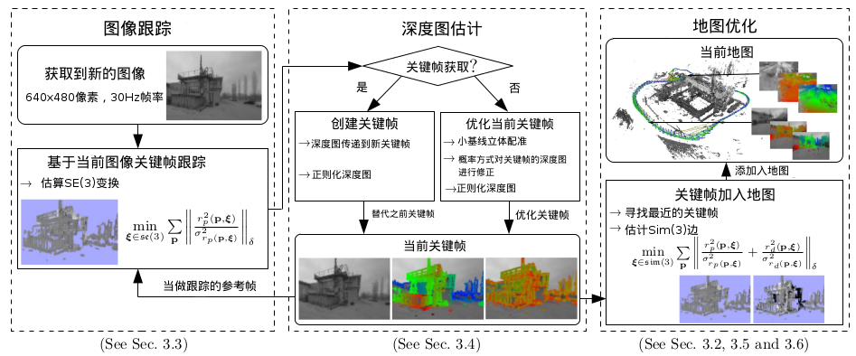示图3: LSD-SLAM算法的整体流程示意图。

图像跟踪流程详见3.3小节， 深度图估计详见3.4小节，地图优化详见3.2，3.5和3.6小节

In practice, the residuals are highly correlated, such that $\mathbf{\Sigma}_{\mathbf{\xi}}$ is only a lower bound - yet it contains valuable information about the correlation between noise on the different degrees of freedom.

实际情况中，残差之间（光度测量误差之间）是高度相关性的（因为我们假设残差之间是独立不相干的变量i.i.d.），使得这个协方差 $\mathbf{\Sigma}_{\mathbf{\xi}}$ 仅仅是个下限（这个补充还需要确认）—但是它仍然包含了噪声之间在不同自由度上的相关性，这一有用信息。(高度相关性作何理解？ 方差下限作何理解？ 感谢和陈创荣的讨论，一种观点认为残差是独立不相干的随机变量，但是实际上这些变量间是应该是相关性的，所以如果相关性的话，方差应该会更大。译者额外添加备注，还需要确认，感谢清华大学高翔博士的指点，建议译者参考2013年Engel的Paper$^*$）

$^*$Semi-Dense Visual Odometry for a Monocular Camera https://vision.cs.tum.edu/_media/spezial/bib/engel2013iccv.pdf

Note that we follow a left-multiplication convention, equivalent results can be obtained using a right-multiplication convention.

注意到，我们这里使用左乘法则，如果使用右乘法则，也可以获得相等的结果。

However, the estimated covariance $\mathbf{\Sigma}_{\mathbf{\xi}}$ depends on the multiplication order – when used in a pose graph optimization framework, this has to be taken into account.

然而，估计协方差 $\mathbf{\Sigma}_{\mathbf{\xi}}$ 取决于乘法的顺序—因此当使用姿态图优化（软件）框架的时候，这一点要考虑进去。

The left-multiplication convention used here is consistent with [23], while e.g. the default type-implementation in g2o [18] assumes right-multiplication.

这里使用的左乘规则和论文[23]是一致的，然而像g2o [18] 姿态图优化（软件）框架，默认的实现类型是使用右乘规则。（请在使用的时候注意，译者额外添加备注）